Area

Area is a concept familiar to all of us from our study of various geometric figures such as rectangles, triangles, and circles. We generally think of area as a number that in some way suggests the size of a bounded region. Of course, we have specific formulas for calculating the areas of simple geometric figures.
Look also at the Fairy Tale - Thoughts for a Wedding Reception.


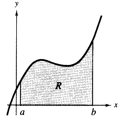
Our problem here is to develop a way to calculate the area of a plane region R, bounded by the x-axis, the lines x = a and x = b, and the graph of a nonnegative continuous function f, as shown in the next Figure.


The solution to this problem is given by the Fundamental Theorem of Calculus and represents one of the most famous discoveries in mathematics. From this theorem we can see that, just as the derivative can be used to find slope, the antiderivative can be used to find area. In anticipation of the connection between antiderivatives and area, we denote the area of the region shown in the previous Figure by

a b f(x) dx

The symbol a b f ( x ) d x   is called the definite integral from a to b, where
a is the lower limit of integration and b is the upper limit of integration.

We will present here the
concept of definite integral involves the notion of the limit of a sum. We give a brief introduction to the notion of representing a definite integral as the limit of a sum. In doing this, we will also discuss a method of approximating definite integrals by the Midpoint Rule. Other approximation methods you can find in the Level II - Numerical Integration.


Approximating the Area of a Plane Region

EXAMPLE
Let f be a function.
f ( x ) = - x 2 + 5
We will try approximate the area of the region lying between the graph of  f(x) and the  x-axis between  x = 0 and  x = 2.

SOLUTION
We will use the five rectangles to approximate this area. Look at the next Figure

We can find the height of the five rectangles shown in the previous Figure by evaluating the function f at the midpoint of each of the following intervals.
[ 0 , 2 5 ] [ 2 5 , 4 5 ] [ 4 5 , 6 5 ] [ 6 5 , 8 5 ] [ 8 5 , 2 ]
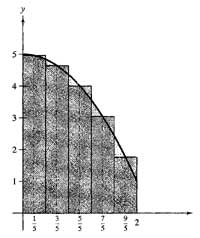
Evaluate f(x) at the midpoints of these intervals

Since the width of each rectangle is 2/5, them sum of areas of the five rectangles is
Area f ( 1 5 ) ( 2 5 ) + f ( 3 5 ) ( 2 5 ) + f ( 5 5 ) ( 2 5 ) + f ( 7 5 ) ( 2 5 ) + f ( 9 5 ) ( 2 5 ) =
= 2 5 [ f ( 1 5 ) + f ( 3 5 ) + f ( 5 5 ) + f ( 7 5 ) + f ( 9 5 ) ] =
= 2 5 [ 124 25 + 116 25 + 100 25 + 76 25 + 44 25 ] =
= 2 125 [ 124 + 116 + 100 + 76 + 44 ] =
= 920 125 = 7.36

For the region in this example we can find the exact area with a definite integral (see also
Fundamental Theorem of Calculus ). That is

Area = 0 2 ( - x 2 + 5 ) d x = [ x 3 3 + 5 x ] 0 2 =
= ( - 8 3 + 10 ) - ( 0 ) = 22 3 7.3333

We call the approximation procedure used in the previous example the
Midpoint Rule. We can apply the Midpoint Rule to the approximate any definite integral - not just those representing area. The basic steps are summerized as follows.

Using the Midpoint Rule
to Approximate a Definite Integral
To approximate the definite integral
a b f(x) dx
by the Midpoint Rule, use the following steps.

   1.  Divide the interval [a,b] into n subintervals, each of width

x = b - a n

   2.  Find the midpoint of each subinterval

M i d p o i n t s = { x 1 , x 2 , x 3 , &dots; , x n }
   3.  Evaluate f at each of these midpoints and form the following sum
a b f ( x ) d x b - a n [ f ( x 1 ) + f ( x 2 ) + f ( x 3 ) + &dots; + f ( x n ) ]