APPROXIMATION and INTERPOLATION CURVES

Approximation (interpolation) is a generating principle, which enables to model connected curve segments from the discrete ordered sets of points in the extended Euclidean space. Intrinsic geometric properties of the modelled curves depend on the form of the polynomial interpolation functions determining the analytic representations of the modelled figures, it means on the values of the coefficients in the powers of the variable u. Required geometric properties of the resulting curve segment determine the conditions for calculation of these coefficients. In general, the interpolation polynomials

Pl_i(u)=a_inuⁿ+a_in-1uⁿ-1+...+a_i1u+a_i0

must satisfy the following condition:
sum of the polynomials related to the real points of the basic figure (in the given order) is equal to 1

           (1)

Analytic representation of the modelled curve segment determined by the ordered n-tuple of points
represented analytically by the map

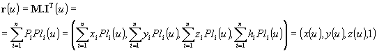
M=( P_i(x_i , y_i , z_i , h_i ) ), i=1, ..., n, where h_i = 0, 1

and created by applying an approximation (interpolation) determined by the interpolation matrix

I(u)=( Pl₁(u) Pl₂(u) ... Pl_n(u) )

is the point function of the required properties on I=<0,1>

We distinguish two different types of modelling:

interpolation - all points of the basic figure are located on the created figure called interpolation curve segment

approximation - all points of the basic figure need not be located on the created figure called approximation curve segment.

Modelling can be applied to the whole ordered set, n-tuple of points, or it can be modelled by parts, while the created curve is composed from elementary curve segments, usually cubic ones. Both modelling methods of curve segments have tsome advantages and some disadvantages.
If we apply the interpolation on the whole n-tuple of points, the resulting curve is of the degree n-1, it has many extremal points (with extremal curvatures in some points, or points of inflection) and usually it is not possible to change its shape locally (in the neighbourhood of some point only), modelling of the curve is not flexible.
In modelling by parts it is important to provide continuity and smoothness of the resulting curve in the common points of the separate adjoining curve segments, by the equality of some elements of the adjoining curve segments basic figures, it means in the input data structure for the computer processing. These data files are usually in the practical applications very large and not easy to convey, and their change is very difficult and inconvinient.
We will speak about several types of modelled curve segments most frequently used in the CAD systems of the computer based design and modelling.

Cubic curve segment is the curve segment with the basic figure in the form of the ordered quadruple of the points in the extended Euclidean space

P_i=(x_i, y_i, z_i, h_i) , for i=0, 1, 2, 3,   where h_i = 0, 1

Generating principle is an approximation (interpolation) determined by the ordered set of cubic interpolation polynomials

Pl_i(u)=a_iu³+b_iu²+c_iu+d_i , for i=0, 1, 2, 3

satifying the condition (1).

1. Ferguson cubic (cubic interpolation curve segment)

Ferguson cubic is the interpolation curve segment determined by the start and the end points and tangent vectors in these points. Interpolation is determined by cubic Hermit polynomials.

Synthetic representation:     ({P₀, P₁, a ₀, a₁}, I(u) )

Analytic representations:

basic figure -   P₀=(x₀, y₀, z₀, 1)  P₁=(x₁, y₁, z₁, 1)
                      a₀=(x_A0, y_A0, z_A0, 0)      a₁=(x_A1, y_A1, z_A1, 0)

map of the curve segment         M =( P₀ P₁ a₀ a₁)

generating principle -         I(u)=(F₀(u), F₁(u), G₀(u), G₁(u)), where

F₀(u)=2u³-3u²+1       F₁(u)= -2u³+3u²        G₀(u)=u³-2u²+u       G₁(u)=u³-u²

are Hermit interpolation polynomials, while

modelled figure -   r(u)=M.I^T(u)= P₀F₀(u)+ P₁F₁(u)+ a₀ G₀(u)+ a₁G₁(u), uÎ<0,1>

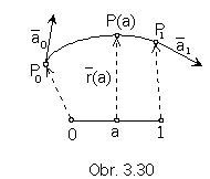
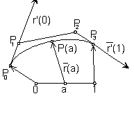
It is valid:               r(0)=P₀     r(1)=P₁     r´(0)=a₀    r´(1)= a₁

The start point of the Ferguson cubic segment is the point P₀, the end point is the point P₁.
Tangent vector in the point P₀ to the curve is the vector a₀, in the point P₁ the vector a₁.
Geometric properties of the modelled curve segment determine the conditions for the calculation of coefficients of the used interpolation polynomials. The name Hermit polynomials is related to the name of the mathematician Hermit, who lived in the 19th century and used these polynomials for the interpolation of functions. Applied generating principle is known as the Hermit cubic interpolation.
Coordinates of the interior points on the Ferguson cubic segment can be calculated from the curve point function for the values of the point curvilinear coordinates in the interval (0,1).

In the majority of the practical applications, the interpolation curve is determined only by the ordered set of real points, which must be located on the resulting curve. Tangent vectors determining the curvatures (flection and torsion) in the given point on the modelled curve segment are inserted empirically, and their choice depends on the skill of the user. These can cause, in general, a rather serious problem in the industrial design and modelling, because tangent vectors influence deeply the shape of the resulting curve segments.
In the more sofisticated CAD systems, there is provided the possibility to determine tangent vectors with respect to the form of the basic figure - the ordered set of real points in the space, so that the resulting interpolation curve has the "quiet flow", it copies the shape of the basic polygon without large extremes.
One of the methods for determination of the tangent vectors in the point on the interpolation curve widely used in the practise is the Akima interpolation.
Let P_i-2 P_i-1 P_i P_i+1 P_i+2 be the part of the basic polygon
determined by the points of the interpolation curve basic figure (Fig. 3. 31).
Akima construction can be used to determine the tangent vector in the point P_i on the curve.
Let us find first points A_i, B_i a C_i, for which the following is valid

P_i-2P_i-1 Ç P_iP_i+1 =A_i

P_i-1P_i Ç P_i+1P_i+2 =B_i

A_iB_i Ç P_i-1P_i+1 =C_i

t_i=P_iC_i , if C_i is the ideal point, then
               

A_iB_i // P_i-1P_i+1 // t_i, | t_i|=| P_i-1P_i+1 |

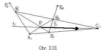
In the first (last) two points of the ordered sequence of points in the basic figure it is necessary to determine tangent vectors by a different method, for example as the tangent vectors to the conic section segment (parabola) passing through the first (last) three points.

A different method to determine tangent vectors is the D-interpolation, in which the tangent vector a in the point P_i is determined as the linear combination of the vectors formed by the given point and two other points of the basic figure,
point P_i-1 (proceeding the tangent point)
and point P_i+1 (succeeding the tangent point) (Fig. 3. 32).

      j=

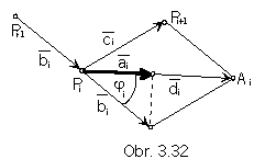
Vector a is the image of the vector b in the orhogonal mapping to the vector of the sum d_i.

Interpolation cubic determined by the basic figure { P₀ P₁ a₀ a₁}, in which the tangent vectors are determined by
the D-interpolation, and for which the generating interpolation polynomials are Hermit ones, is called the D-spline cubic.

Owerhauser cubic is the interpolation curve determined by the ordered n-tuple of points and Hermit interpolation, while tangent vectors to the curve are determined in the start point and in the end point, only.

2. Bézier cubic (cubic approximation segment)

Bézier cubic is the approximation curve determined by the four real points in the basic figure. Approximation is determined by Bernstein cubic polynomials.

Synthetic representation:     ({P₀ ,P₁ ,P₂ ,P₃}, I(u))

Analytic representations:

basic figure -     P_i=(x_i, y_i, z_i, 1) , for i=0,1,2,3

map of the curve segment     M=(P₀ P₁ P₂ P₃)

generating principle -     I(u)=(Be₀₃(u) Be₁₃(u) Be₂₃(u) Be₃₃(u)), where

Be₀₃(u)=(1-u)    Be₁₃(u)=3u(1-u)²     Be₂₃(u)=3u²(1-u)    Be₃₃(u)=u³

are Bernstein approximation polynomials, while .

modelled figure    r(u)=M.I(u)=P₀Be₀₃(u)+P₁Be₁₃(u)+P₂Be₂₃(u)+P₃Be₃₃(u), uÎ<0,1>

It is valid:     r(0)= P₀    r(1)=P₃    r(0)=3 P₀ P₁    r(1)=3 P₂ P₃

The start point of the curve segment is the point P₀ and tangent vector to the curve segment in this point is the three multiple of the vector in the first side of the basic polygon - 3P₀P₁. The end point is the point P₁, tangent vector in this point is the three multiple of the vector in the last side of the basic polygon - 3P₂P₃. Given geometric properties of the modelled cubic curve segment are provided by the used Bernstein polynomials, called by the Russian mathematician Bernstein, who used them for the approximation of functions ulready in the year 1912.
The general formula for calculation of these polynomials of degree n is

, for i=0,...,n, where n is the degree.

Homogeneous coordinates of the interior points on the Bézier cubic with the curvilinear coordinates in the interval (0,1) can be calculated from the point function.
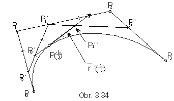
Point on the Bézier cubic can be constructed by the algorithm Boor - de Casteljau (Fig. 3. 34).

Let a=1/3 be the curvilinear coordinate of the point on the cubic in the interval (0,1).
In the one third of the length from the start point on each of the sides of the basic polygon P₀P₁ , P₁P₂ , P₂P₃
there are located points P₀', P₁', P₂' determining new basic figure, which can be reduced by the same construction up to one line segment P₀''P₁''
and then to one point P(1/3) located on the Bézier segment.
Tangent vector in this point is determined as
r(1/3)=P₀P₁.

3. Coons B-spline cubic (cubic approximation curve segment)

Coons B-splie cubic is the approximation curve determined by four real points in the basic figure. Approximation is defined by Coons cubic polynomials (obr. 3.35).

Synthetic representation:     ({P₀, P₁, P₂, P₃}, I(u))

Analytic representations:

basic figure -     P_i=(x_i, y_i, z_i, 1) , for i=0,1,2,3

map of the curve segment     M=(P₀ P₁ P₂ P₃)

generating principle - I(u)=(Co₀₃(u) Co₁₃(u) Co₂₃(u) Co₃₃(u)), where

Co₀₃(u)=            Co₁₃(u)=


Co₂₃(u)=            Co₃₃(u)=

are Coons approximation polynomials, while .

modelled figure -   r(u)=M.I^T(u)=P₀Co₀₃(u)+P₁Co₁₃(u)+P₂Co₂₃(u)+P₃Co₃₃(u), uÎ<0,1>

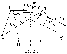
It is valid :      r(0)=((P₀+P₂)/2+2P₁)/3     r(0)=(P₂-P₀)/2

                      r(1)=((P₁+P₃)/2+2P₂)/3    r(1)=(P₃-P₁)/2

The start point of the curve segment is the anticentre of the gravivity in the triangle P₀P₁P₂ located on the median passing through the vertex P₁ to the centre of the side P₀P₂ in one third of its size from the vertex P₁ .
The end point of the curve segment is the anticentre of the gravity in the triangle P₁P₂P₃ located on the median passing through the vertex P₂ to the centre of the side P₁P₃ in one third of its size from the vertex P₂ .
Tangent vectors in these points are collinear to the vectors P₀+P₂ , P₁+P₃.
Geometry of the modelled curve segment is provided by Coons polynomials called after the American computer graphician Coons, which are special types of B-spline cubic polynomials.

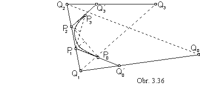
The fact, that the modelled curve does not contain any point of the basic figure and in modelling it is not clear, where are located the start and the end points of the curve segment, causes a certain disadvantage in the practical usage of B-spline cubics in the computer aided design.
The input basic figure, an ordered quadruple of real points {P₀ , P₁ , P₂ , P₃}, can be substituted by a new basic figure
- suplementary basic polygon {Q₀ , Q₁ , Q₂ , Q₃}, which can be constructed in the way,
that points P₀ and P₃ be the start and the end points of the approximation B-spline curve segment
with the basic figure in the new suplementary basic polygon {Q₀ , Q₁ , Q₂ , Q₃},
curve can be "prolonged" to the points P₀ and P₃ (Fig. 3.36).

|Q₁P₁|=|P₁P₂|=|P₂Q₂|

|Q´₀P₀|=|P₀P₁|

|Q₀Q´₀|=2|Q´₀Q₁|

|Q´₃P₃|=|P₃P₂|

|Q₃Q´₃|=2|Q´₃Q₂|

In all forthcoming types of modelled curves it is possible to reach the change in the shape of the curve only by the change of elements in the basic figure, which represent the input data file for the computer processing. This file is in practical situations very large one and not easy to convey, which limits the modelling power of the user. Change of the intrinsic properties of the modelled curve segment can be also reached by the change of the generating principle, it means by the change of the used polynomial functions, having the possibility to change cofficients of these polynomials through several input parameters.

4. b-spline cubic (cubic approximation curve segment)

b-spline cubic is the approximation curve determined by the ordered quadruple of real points in the space. Approximation is defined by b-spline cubic polynomials.

Synthetic representation:  ({P₀ , P₁ , P₂ , P₃}, I(u))

Analytic representations:

basic figure -     P_i=(x_i, y_i, z_i, 1) , for i=0,1,2,3

map of the curve segment     M=(P₀ P₁ P₂ P₃)

generating principle - I(u)=(Ba₀₃(u) Ba₁₃(u) Ba₂₃(u) Ba₃₃(u)), where

Ba₀₃(u) =

Ba₁₃(u) =

Ba₂₃(u) =

Ba₃₃(u) =          

are b-spline approximation polynomials.

modelled figure -      r(u)=M.I^T(u)=P₀ Ba₀₃(u)+P₁Ba₁₃(u)+P₂Ba₂₃(u)+P₃Ba₃₃(u), uÎ<0,1>

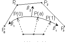
Coefficients of b-spline polynomials are functions of two real parameters, influencing the intrinsic properties of the modelled curve segments.

Parameter b₁ - tension influences the position of the strat and the end points of the curve segment, it
"takes" the curve to the first, or to the last point of the basic figure.

Parameter b₂ - torsion influences the first curvature of the modelled curve segment in its interior points,
"stretches" ("looses") the curve towards (from) the side P₁P₂ of the basic figure.
If b₁=1 and b₂=0, we receive Coons B-spline polynomials.

5. Rational cubics (cubic approximation curve segments)

Rational cubic is the approximation curve determined by the ordered quadruple of real points in the space and positive weights of these points (chosen representants from the class of homogeneous coordinates of points). Weight of the point expresses the scale, in which the point has to influence the shape of the modelled curve. Approximation is determined by cubic polynomials.

Synthetic representation:     ({h₀P₀ , h₁P₁ , h₂P₂ , h₃P₃}, I(u))

Analytic representations:

basic figure -     P_i=h_i(x_i, y_i, z_i, 1), h_i>0, for i=0,1,2,3

map of the curve segment          M=(h₀P₀ h₁P₁ h₂P₂ h₃P₃)

generating principle -     I(u)=(Pl₀₃(u) Pl₁₃(u) Pl₂₃(u) Pl₃₃(u)), where

    Pl_i3(u) for i=0,1,2,3 are approximation cubic polynomials - Bernstein, B-spline, b-spline, for which

modelled figure -     rational extension of the cubic approximation curve
(Bézier, Coons, B-spline, b-spline) represented by the point function

R(u)=M.I^T(u)= ,

where H(u)= is the weight function, non-zero for uÎ<0,1>.

Rational approximation cubic curve segment is for uÎ<0,1> determined by the rational point function

With respect to the size of the weight of each point in the basic figure the shape of the modelled curve segment can be modified.
For values h₀= h₁= h₂= h₃ the modelled curve segment is related Bézier, Coons B-spline or b-spline cubic segment.

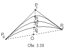
Segments of conic sections can be modelled as approximation Bézier rational quadratic segments (Fig. 3. 38).

Synthetic representation:        ({h₀P₀ h₁P₁ h₂P₂ }, I(u))

Analytic representations:

basic figure -     P_i=h_i(x_i, y_i, z_i,1), h_i>0, for i=0,1,2

map of the curve segment      M=(h₀P₀ h₁P₁ h₂P₂)

generating principle -     I(u)=(Be₀₂(u) Be₁₂(u) Be22(u)), where

    Be₀₂(u)=(1-u)²        Be₁₂(u)=2u(1-u)        Be₂₂ (u)=u²

    are Bernstein approximation polynomials of the degree two