Visualisation
Mathematica offers many different ways for drawing graphics by setting formulas or tables of data. There are static and animated graphics as well as sound. Graphic images can be shown from different perspectives and in a different kind by using the appropriate options and special build-in functions as Show, RealTime etc.
Example 1. A two dimensional graphics demands a given function formula and an interval. There is a wide range of options and settings for formatting. Two graphics of the function Sin[x] in the interval [ -2π, 2π ] are shown below. The graphics g1 is with default options and the graphics g2 has four changes - frame size, style (colour and line thickness) and ratio of ![]() between the axes measures.
between the axes measures.
![g1 = Plot[Sin[x], {x, -2π, 2 π}] RowBox[{g2, =, RowBox[{Plot, [, RowBox[{Sin[x], ,, ... , ,, RowBox[{Thickness, [, 0.02, ]}]}], }}]}], ,, , RowBox[{AspectRatio, , 1.}]}], ]}]}]](HTMLFiles/index_2.gif)
![[Graphics:HTMLFiles/index_3.gif]](HTMLFiles/index_3.gif)
![]()
![[Graphics:HTMLFiles/index_5.gif]](HTMLFiles/index_5.gif)
![]()
Example 2. Simultaneous drawing of several graphics is done by using the function Show[ ].
![]()
![[Graphics:HTMLFiles/index_8.gif]](HTMLFiles/index_8.gif)
![]()
![[Graphics:HTMLFiles/index_10.gif]](HTMLFiles/index_10.gif)
![]()
Example 3. A two dimensional list plot needs a given table with point coordinates. Typically this is best done with lists. Here is a list of points and corresponding graphics with options.
![]()
![[Graphics:HTMLFiles/index_13.gif]](HTMLFiles/index_13.gif)
![]()
Example 4. The parametric curve demands formulas for calculating the coordinates { x, y } and the interval of the parameter. Here the option AspectRatio is also added in order to set the ratio ![]() . In this case a Fibbonacci number is chosen for the golden ratio - the constant GoldenRatio equal to 0.618... :
. In this case a Fibbonacci number is chosen for the golden ratio - the constant GoldenRatio equal to 0.618... :
![]()
![[Graphics:HTMLFiles/index_17.gif]](HTMLFiles/index_17.gif)
![]()
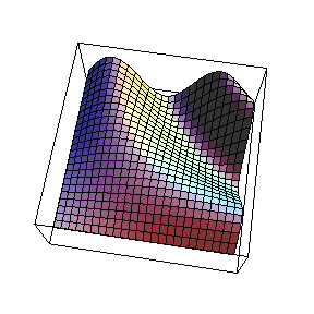
Example 5. A three dimensiaonal graphics in Cartesian coordinates at a given formula and interval for the two coordinates. The viewpoint for the same graphics is then changed.
![]()
![[Graphics:HTMLFiles/index_20.gif]](HTMLFiles/index_20.gif)
![]()
![[Graphics:HTMLFiles/index_22.gif]](HTMLFiles/index_22.gif)
![]()
Example 6. Mathematica has the capability for visualization in real time by using the fastest possible way to calculate and compile for instant visualization of the result. Here we show how this is done. The package <<RealTime3D must be introduced. You can drag the graphics by the mouse and set the velocity of moving it. The <<Default3D removes the action of RealTime.
![<<RealTime3D` Show[dd] <<Default3D`](HTMLFiles/index_24.gif)

![]()
Example 7. A contour graphics of the previous function is easy to plot:
![]()
![[Graphics:HTMLFiles/index_28.gif]](HTMLFiles/index_28.gif)
![]()
Example 8. The parametric three-dimensional graphics of a function use set formulas for calculating the coordinates { x, y, z} and parameter variation of intervals. This type of graphics offers the possibility of using cylindrical, spherical and other coordinates.
![pp2 = ParametricPlot3D[{u * Sin[t], u * Cos[t], t/3}, {t, 0, 9}, {u, -1, 1}, BoxedFals ... xesNone, ViewPoint {1, 2, 4}] pp4 = Show[pp2, pp3 , ViewPoint {3, 2, -1}]](HTMLFiles/index_30.gif)
![[Graphics:HTMLFiles/index_31.gif]](HTMLFiles/index_31.gif)
![]()
![[Graphics:HTMLFiles/index_33.gif]](HTMLFiles/index_33.gif)
![]()
![[Graphics:HTMLFiles/index_35.gif]](HTMLFiles/index_35.gif)
![]()
Example 9. More complex objects can be constructed by using either ready 2D or 3D primitives, or the ones we created, in other words, ready basic objects such as segment, circle, partial ellipse etc. Here a table with coordinates of points in the plane is created. The first command ends with semicolon in order to hide the numbers while the second line shows the coordinates of only the first 4 points. The 3rd line draws the derived points.
![gr = Flatten[Table[Point[{p/q, q}], {q, 100}, {p, q - 3}]] ; Take[%, 4] Show[Graphics[gr, FrameTrue]]](HTMLFiles/index_37.gif)
![]()
![[Graphics:HTMLFiles/index_39.gif]](HTMLFiles/index_39.gif)
![]()
Example 10. The generation of an animated graphics is done by a little programme containing a cycle. To start the animation the graph must be double clicked. The animation is stopped by clicking outside the graphics.
![]()
Example 11. Another animated graphics.
![RowBox[{RowBox[{Do, [, RowBox[{RowBox[{ParametricPlot3D, [, RowBox[{{Cos[i π/50] Cos[2 ... , ,, RowBox[{{, RowBox[{RowBox[{-, 1.1}], ,, 1.1}], }}]}], }}]}]}], ]}], ,, {i, 0, 25}}], ]}], ;}]](HTMLFiles/index_64.gif)
Example 12. The generation of sound is done with the function Play. That way the formulas can play any given sound. To hear the sound we must have a computer with an audio device and double click on the graphics.
![Play[Sin[(π t)/2] ∑_ (ν = 0)^24If[ν/12<t<ν/12 + 1/4, 1/24 ? ... (3 + 2 ν - 24 t)^2) ν Sin[1625 ν t - 13000 t], 0], {t, 0, 2}, PlayRangeAll]](HTMLFiles/index_92.gif)
![[Graphics:HTMLFiles/index_93.gif]](HTMLFiles/index_93.gif)
![]()
Created by Mathematica (October 6, 2007)