BG_1_students guide chapter

The least-squares method for approximation of data
using Mathematica

Background

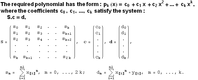
$Given : A table of the function y = f (x) : { x_1, y_1}, ..., { x_n1, y_n1} .$

The required polynomial has the form : p_k (x) = c_0 + c_1x + c_2x^2 +.. ... . . . 2k k k

The mean squared error is : δ_k = (Underoverscript[∑, i = 1, arg3] (f (x_i) - p_k (x_i))^2)^(1/2) .

RowBox[{RowBox[{RowBox[{RowBox[{RowBox[{RowBox[{RowBox[{RowBox[{RowBox[{RowBox[{RowBox[{RowBox ... 3, , using, , the, , polynomial .}], FontFamily -> Arial, FontSize -> 18, FontWeight -> Bold]}]

$f[xx_] := xx + Sin[xx^2] RowBox[{RowBox[{a, =, 1.}], ;, RowBox[{b, =, 2.}], , ;}] gf = Plot[f[xx], {xx, a, b}]$

[Graphics:HTMLFiles/index_11.gif]

n1 = 11 ; h = (b - a)/(n1 - 1) ; Print["Step h= ", h] x = Table[a + h * ... stPlot, [, RowBox[{xy, ,, RowBox[{PlotStyle, , RowBox[{PointSize, [, 0.02, ]}]}]}], ]}]}]

[Graphics:HTMLFiles/index_19.gif]

b) We calculate all the sums needed for the LSM of the first degree, we solve the c ... lve[ ] Mathematica command and extract the coefficients of the polynomial - c0 and c1 :

s0 = n1 ; s1 = Underoverscript[∑, i = 1, arg3] x_〚i〛 ; s2 = Un ... Solve[S, d] c0 = c_〚1〛_〚1〛 c1 = c_〚2〛_〚1〛

We define the polynomial of best approximation of the first degree of LSM as a function and dr ... raphs of the table of f (x) and its approximation p1 (x) :

$p1[xx_] := c0 + c1 * xx gp1 = Plot[p1[xx], {xx, a, b}, PlotStyleHue[.6]] Show[gy, gp1]$

[Graphics:HTMLFiles/index_30.gif]

[Graphics:HTMLFiles/index_32.gif]

δ_1 = (Underoverscript[∑, i = 1, arg3] (f[x_〚i〛] - p1[x_〚i〛])^2)^(1/2)

StyleBox[RowBox[{RowBox[{d), , The, , approximate, , absolute, , value, , of, ... ;only on a table of measured values :}], FontFamily -> Arial, FontSize -> 18., FontWeight -> Bold]

Conclusion: The obtained error is obviously large as can also be seen from the graphs of both functions. An approximation with a polynomial of a higher degree can be found.

StyleBox[RowBox[{RowBox[{RowBox[{RowBox[{RowBox[{RowBox[{RowBox[{RowBox[{Problem, , 2., ... , f, RowBox[{RowBox[{(, 1.33, )}], .}]}], FontFamily -> Arial, FontSize -> 18, FontWeight -> Bold]

a) We calculate all the sums needed for LSM of the second degree, we solve the corresponding s ... ing LinearSolve and extract the coefficients of the polynomial, which we mark with v0, v1 and v2 :

s0 = n1 ; s1 = Underoverscript[∑, i = 1, arg3] x_〚i〛 ; s2 = Un ... 4;1〛 v1 = c_〚2〛_〚1〛 v2 = c_〚3〛_〚1〛

We define the 2nd degree polynomial providing best approximation according to the LSM, as a fu ... ltaneously display both the graphs of the table of f (x) and its approximation p2 (x) :

$p2[xx_] := v0 + v1 * xx + v2 * xx^2 gp2 = Plot[p2[xx], {xx, a, b}, PlotStyleHue[.3]] Show[gy, gp2]$

[Graphics:HTMLFiles/index_54.gif]

[Graphics:HTMLFiles/index_56.gif]

δ_2 = (Underoverscript[∑, i = 1, arg3] (f[x_〚i〛] - p2[x_〚i〛])^2)^(1/2)

RowBox[{StyleBox[RowBox[{p2, [, 1.33, ]}], FontColor -> GrayLevel[0.]], }] RowBox[{RowBox[{a ... wBox[{p2, [, 1.33, ]}]}], ]}]}], ;, , Print[" The test absolute error now is=", aer]}]

Conclusion: The derived errors and aer are obviously still large but are more acceptable than the former approximation (compare the graphs of the two functions). An approximation with a polynomial of an even higher degree can be found.

StyleBox[RowBox[{RowBox[{RowBox[{RowBox[{RowBox[{RowBox[{RowBox[{RowBox[{Problem, , 3., ... , RowBox[{RowBox[{(, 1.33, )}], ., }]}], FontFamily -> Arial, FontSize -> 18, FontWeight -> Bold]

a) We calculate all the sums needed for LSM of the fifth degree, we solve the algebraic linear ... act the coefficients of the polynomial, which we mark with z0, z1, z2 , z3, z4 and z5 :

s0 = n1 ; s1 = Underoverscript[∑, i = 1, arg3] x_〚i〛 ; s2 = Un ... 2315; ; z4 = c_〚5〛_〚1〛 ; z5 = c_〚6〛_〚1〛 ;

We define the best 5th degree approximating polynomial as a function and plot its graph . &nbs ... ltaneously display both the graphs of the table of f (x) and its approximation p5 (x) :

$p5[xx_] := z0 + z1 * xx + z2 * xx^2 + z3 * xx^3 + z4 * xx^4 + z5 * xx^5 gp5 = Plot[p5[xx], {xx, a, b}, PlotStyleHue[.8]] Show[gy, gp5]$

[Graphics:HTMLFiles/index_73.gif]

[Graphics:HTMLFiles/index_75.gif]

δ_5 = (Underoverscript[∑, i = 1, arg3] (f[x_〚i〛] - p5[x_〚i〛])^2)^(1/2)

RowBox[{StyleBox[RowBox[{p5, [, 1.33, ]}], FontColor -> GrayLevel[0.]], }] RowBox[{RowBox[{a ... Box[{p5, [, 1.33, ]}]}], ]}]}], ;, , Print[" The test absolute error now is=", aer5]}]

Conclusion: The derived error and the test absolute error are now quite satisfactory.

[Graphics:HTMLFiles/index_88.gif]

Created by Mathematica (May 22, 2008)