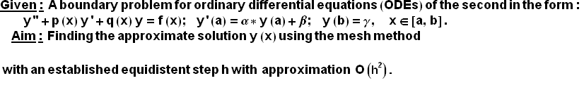
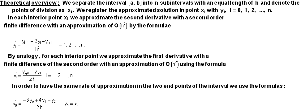
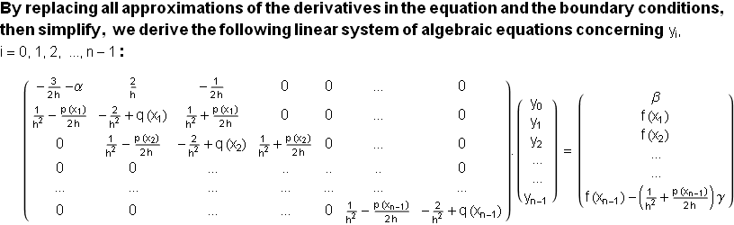
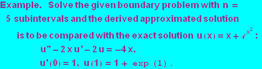
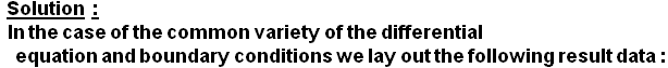
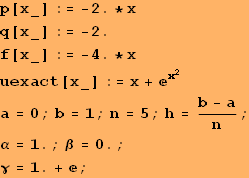
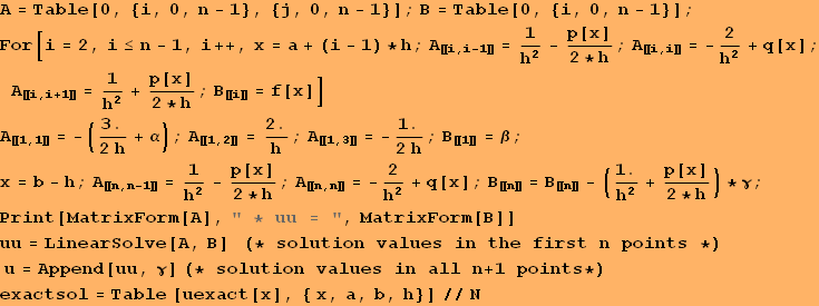
Mesh method for solving boundary value problem of the mixed type using Mathematica

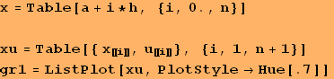
Anotation        

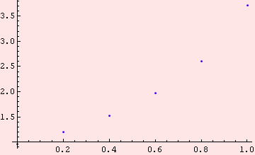
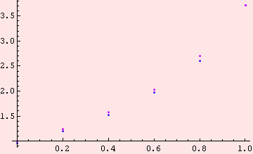
Graphic representation of the solution  

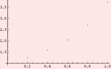
Comparison with the exact solution and real errors

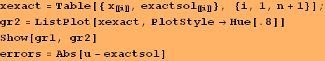
Conclusion
Since in this example h = 0.2 and the approximation is of the order approximate to 0.04.
The real error of the next upper line is 0.1. That is explained with the upper boundary of the derivative of the third order of the exact solution (see more detailed theory).
Recommendation. In order to supply the required error for an arbitrary problem we may reduce the step h until two consecutive approximations in their respective  points match the needed accuracy.

Created by Wolfram Mathematica 6.0  (21 September 2008)