Fourth-order Runge-Kutta Method using Mathematica
![]()
Аnotation


![]()

![]()

![]()
![]()
![]()
![]()
![]()
![]()
![]()
![]()

| 1 | 1. |
| 1.1 | 1.32532 |
| 1.2 | 1.70253 |
| 1.3 | 2.13338 |
| 1.4 | 2.61947 |
| 1.5 | 3.16227 |
Conclusion: The solution derived using the Runge-Kutta method O(![]() ) is in the form of a table of the variable function y(x), shown in the second column of the table above. Since the local apriori error of the method is O(
) is in the form of a table of the variable function y(x), shown in the second column of the table above. Since the local apriori error of the method is O(![]() ) (or global error is O(
) (or global error is O(![]() ) ) and here h=0.1, then these solutions must be rounded to five symbols after the decimal point.
) ) and here h=0.1, then these solutions must be rounded to five symbols after the decimal point.
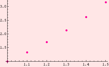
Graphic of the solution
![]()

| Created by Wolfram Mathematica 6.0 (22 September 2008) |