NOTES ON GEOMETRY OF ELEMENTARY SOLID CELLS

1. Introduction

Solid Geometry seems to be one of the topics presented in almost all courses of geometry on all levels of education, in a different range and using appropriate means. Almost all objects we meet or create (engineers especially) in the real world to make it a better place for living are solids. Different sciences try to describe precisely their properties - physical, chemical, biological, etc., in order to state laws of the solids behaviour upon certain conditions in a defined system. Geometric properties, that characterise the shape and the solid interior, are very often neglected, or their are mentioned only very briefly.

The course of geometry at the technical university should take into the consideration the fact that graduates from these schools will use in their everyday work models of 3D objects - solids. They will create them using different methods of modelling and therefore they should understand the relations between different representations of these geometric figures and they must be able to calculate their basic geometric characteristics. New modelling methods - computer aided geometric design - must be incorporated into the course. One of the possibilities suggested in the paper is to model and represent solids on the base of their creative laws using methods of Creative geometry.

Let the Creative space be an ordered pair K=(U, G), where U is a set of figures in the space (non-empty subsets of the extended Euclidean space PE₃) and G = GP(PE₃) È I is a set of generating principles, while GP(PE₃) is a group of all projective transformations of PE₃ and I is a set of interpolations. Solid S (a non-empty three-parametric subset of PE₃ ) is in the Creative space K synthetically represented by its creative representation in thye form of an ordered pair (U, G), where UÎU is a basic figure) and GÎG is a generating principle such, that applying the generating principle G on the basic figure U we obtain the created solid S.

Generating principle G in the form of a geometric transformation or a class of geometric transformations provide modelling of solids that are homogeneous, i.e. the interior points of solid are uniformly distributed. This is usually implicitly assumed in the case of solids defined by their incidence structure describing order and incidence of all elements (vertices, edges, facets) forming the boundary of solids as the three-dimensional subsets of PE₃. In this case we even restrict our considerations on polyhedra, while using creative representation more complex shaped figures and solids with "curve-like" edges can be modelled.

The possibility to describe and to control the feature of an inhomogeneous distribution of points in a solid is provided in the case of its modelling as an interpolated figure, using its creative representation with the generating principle is an interpolation.

Analytic representation of the solid S is a point function

s(u,v,w) = (x(u,v,w), y(u,v,w), z(u,v,w), h(u,v,w))

defined on the region W Ì R³ (where x, y, z, h are homogeneous coordinate functions at least once differentiable on W), which is a locally homeomorphic mapping of W on solid S, and h(u,v,w)=0 for points at infinity. For W = [0,1]³ we speak about solid cell (Fig. 1), that corresponds to the notion of a curve segment or a surface patch. Composite solid can be composed from several elementar cells.

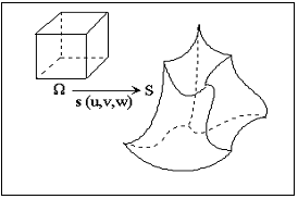
Fig.1

The first fundamental form of the solid is the square of the solid point function total differential

(ds) ²=(s_u du + s_v dv + s_w dw) ²=

= s_u²du²+2s_us_v dudv+s_v²dv²+2s_us_w dudw+2s_vs_w dvdw+s_w²dw² =

= j₁(u,v) + j₁(u,w) + j₁(v,w) - j = F₁

and can be expressed as the sum of the first fundamental forms j₁(u,v), j₁(u,w) and j₁(v,w) of the solid isoparametric patches subtracted by the sum j of the first fundamental forms of the solid parametric segments.

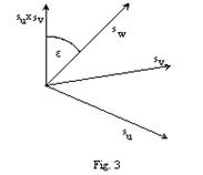
The triple scalar product s of the tangent vectors to the solid cell isoparametric segments (partial derivatives s_u , s_v , s_w of the solid point function ) can be determined by the coefficients of the solid first fundamental form and the volume V of the solid cell can be calculated.

where (Fig. 3)

e =úØ(s_u ´ s_v ), s_wú , j =úØ(s_u ´ s_w ), s_vú, y =úØ(s_v ´ s_w ), s_uú

For e, j, y= 0, p is h=3 and we speak about non-dense distribution of points in the direction of the respective tangent vector to the cell isoparametric segment. Geometric interpretation is obvious, tangent vectors form the orthogonal tangent trihedron. For extreme values of angles e, j, y = the value of h streams to infinity and we speak about dense distribution of points in the direction of the respective tangent vector.

The second mixed partial derivatives of the solid point function are twist vectors to the solid isoparametric patches - s_uv , s_vw , s_uw . The third mixed partial derivative s_uvw (the density vector of the solid point function) fors with the twist vectors the second fundamental form of the solid, that can be used for calculations of the homogeneity of the interior point distribution.

2. Modelling of solid cells

Creative representation of a solid cell can be in 3 types of the available forms.

Type 1. (solid cell, geometric transformation)

Basic figure is an elementary solid cell represented analytically by the point function in three variables differentiable on the region [0,1]³

r(u, v, w) = (x(u, v, w), y(u, v, w), z(u, v, w), 1)

Generating principle is in the form of a geometric transformation represented by a regular square matrix of the rank 4

T=(a_ij), for i, j=1, 2, 3, 4

Created solid cell is analytically represented by a point function differentiable on the region [0,1]³

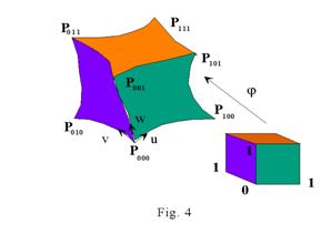
s(u, v, w) = r(u, v, w) .T

In the Fig. 4 there is the image of a unit cube in the non-linear mapping.

Type 2. (surface patch, class of geometric transformations)

Basic figure is a surface patch analytically represented by a point function

p(u, v) = (x(u, v), y(u, v), z(u, v), h(u, v))

at least once differentiable on the region [0,1]², h(u, v)=0 for the surface patch ideal points.

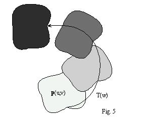
Generating principle is a class of geometric transformations analytically represented by a regular square matrix function of rank 4 in one real variable w , differentiable on [0,1]

T(w)=(a_ij(w)), i, j=1,2,3,4

Modelled solid cell (Fig. 5) is analytically represented by the point function

s(u, v, w) = p(u, v) .T(w)

differentiable on the region W = [0,1]³.

Translation solids

Class of translations, that is a generating principle in the creative representation of translation solids is analytically represented by the matrix function T(w) differentiable on [0,1] together with the first derivative T´(w)

Point function of the created translation cell can be determined as follows

s(u, v, w) = p(u, v) .T(w) = (x(u, v), y(u, v), z(u, v), 1) .T(w) =

= (x(u, v)+a₄₁ (w), y(u, v)+a₄₂ (w), z(u, v)+a₄₃ (w), 1)

Density vector of the translation solid that is defined by the density function in the form of the third mixed triple partial derivative of the solid point function

s_uvw(u, v, w) = p_uv(u, v) .T´(w) = (x_uv(u, v), y_uv(u, v), z_uv(u, v), 0) .T´(w) = 0

is a constant zero vector in all points of the translation solid, therefore it is homogeneous with respect to the direction of all three parameters u, v, w.

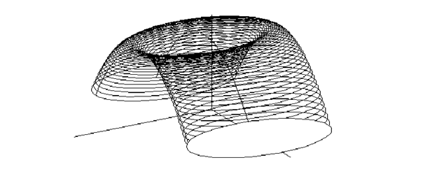
Fig. 6

In the Fig. 6, there is the illustration of the translation solid cell created from the basic figure in the planar region with the boundary in an ellipse by the translation movement with the trajectory in the parabolic segment, while in the Fig. 7 the trajectory is a sinusoid.

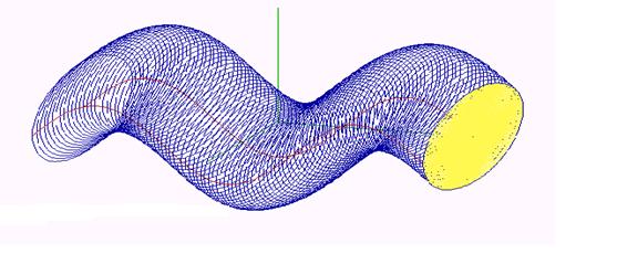
Fig. 7

The first differential form of the translation solid is in the form

j₁(u, v, w) = p_u(u, v).T(w)du²+ p_v(u, v).T(w)dv²+p(u, v).T´(w)dw²

For the special type of the translation functions ^ja(w) for j=1,2,3, w`[0,1] in linear functions we speak about cylinder (prism), that can be created by shifting a basic figure - a surface patch (n-gon) on a trajectory in the form of an oriented line segment

AB = (¹a(1), ²a(1), ³a(1),1)-(¹a(0), ²a(0), ³a(0),1) = (¹a(1)-¹a(0), ²a(1)-²a(0), ³a(1)-³a(0),0)

Solids of revolution

Class of revolutions (e.g. about the coordinate axis z by angles from the interval [0,a]), that is in the place of the generating principle in the creative representation of the solids of revolution is analytically represented by a matrix function R(w) differentiable on [0,1] (together with the first derivative R´(w))

Point function of the created cell of revolution can be expressed as follows

s(u, v, w) = p(u, v) .R(w) = (x(u, v), y(u, v), z(u, v), 1) .R(w) =

= (x(u, v)cosaw - y(u, v)sinaw, x(u, v)sinaw + y(u, v)cosaw, z(u, v), 1)

Illustration of the solid of revolution created from the basic surface patch in the form of a planar region with the boundary in the asteroid by the revolution movement about the coordinate axis z is in the Fig. 8.

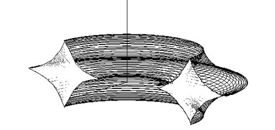
Fig. 8

Density vector of the solid of revolution in the form

s_uvw(u, v, w) = p_uv(u, v) .R´(w) = (x_uv(u, v), y_uv(u, v), z_uv(u, v), 0) .R´(w) =

= a(- x_uv(u, v)sinaw - y_uv(u, v)cosaw, x_uv(u, v)cosaw - y_uv(u, v)sinaw, 0, 0)

is the vector with the zero third coordinate for all points of the solid of revolution, therefore the solid of revolution is homogeneous with respect to the direction of the variable w related to the revolution about the coordinate axis z.

The first differential form of the solid of revolution has the form

j₁(u, v, w) = (p_u(u, v) .R(w)du +p_v(u, v) .R(w)dv +p(u, v) .R´(w) dw)² =

= (x_u² + y_u² + z_u² ) du² +(x_v² + y_v² + z_v ² ) dv² + a² (x² + y²) dw² +

+ 2(x_u x_v + y_u y_v + z_u z_v) du dv + 2a(x y_u - x_u y) du dw + 2a(x y_v - x_v y) dv dw

For the basic surface patch in the form of a planar region with the boundary in a conic section (circle, ellipse, parabola, hyperbola) and axis of the generating movement of revolution in the axis of this conic section, the generated solid is a ball, an ellipsoidal, parabolic, or hyperbolic solid of revolution, resp. a part of it. Toroidal solids can be created as well, when the axis of revolution movement is not incident with the basic circle centre.

Helical solids

Helical movement (e.g. with the axis in the coordinate axis z, the pitch v and angles of revolution in the interval [0,a]), is the generating principle of the helical solids analytically represented by a regular square matrix function S(w) differentiable on [0,1] (together with the first derivative S´(w))

Point function of the created helical solid cell can be derived as follows

s(u, v, w) = p(u, v) . S(w) = (x(u, v), y(u, v), z(u, v), 1) . S(w) =

= (x(u, v)cosaw - y(u, v)sinaw, x(u, v)sinaw + y(u, v)cosaw, z(u, v)+arw, 1)

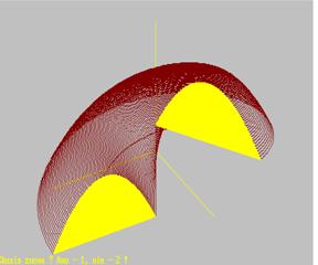
Fig. 9

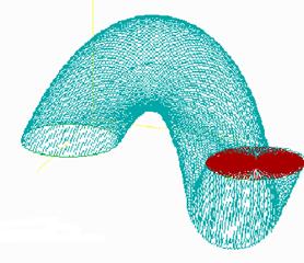
Fig. 10

In the Fig. 9 there is the illustration of the helical solid created from the basic planar region with the boundary in a parabolic arc that is subdued to the helical movement about the coordinate axis z. Moving an ellipsoidal planar region by the helical movement about the coordinate axis y a helical solid shown in the Fig. 10 can be created.

Density vector of the helical solid expressed as

s_uvw(u, v, w) = p_uv(u, v) .S´(w) = (x_uv(u, v), y_uv(u, v), z_uv(u, v), 0) .S´(w) =

= a(- x_uv(u, v)sinaw - y_uv(u, v)cosaw, x_uv(u, v)cosaw - y_uv(u, v)sinaw, 0, 0)

is a vector with the zero third coordinates for all points of the helical solid, therefore the solid is homogeneous with respect to the direction of the variable w related to the helical movement about the coordinate axis z.

The first differential form of the helical solid is in the form

j₁(u, v, w) = (p_u(u, v) .S(w) du + p_v(u, v) .S(w) dv + p(u, v) .S´(w) dw)² =

= (x_u² + y_u² + z_u²) du² + (x_v² + y_v² + z_v)² dv² + a²(x² + y² + r²) dw² +

+ 2(x_u x_v + y_u y_v + z_u z_v) du dv + 2a(x y_u - x_u y + z_u r) du dv + 2j(x y_v - x_v y + z_v r)dv dw

Homothetical solids

Class of homotheties with the centre in the point V=(a,b,c,1) and coefficient k¹0, that is the generating principle for the homothetical solids, is analytically represented by a regular square matrix function H(w) differentiable on [0,1] (together with the first derivative H´(w))

Point function of the created homothetical solid can be expressed as follows

s(u, v, w) = p(u, v) .H(w) = (x(u, v), y(u, v), z(u, v), 1) .H(w) =

= (x(u, v)(1-kw)+akw, y(u, v)(1-kw)+bkw, z(u, v)(1-kw)+ckw, 1)

There is the illustration of the conical frustrum created from the basic planar region bounded by a Steiner hypocycloid, in the Fig. 11, and a doubled conical solid created from the basic planar region with the boundary in the Cardiod in the Fig. 12.

Density vector of the homothetical solid that can be derived from the function

s_uvw(u, v, w) = p_uv(u, v) .H´(w) = -k(x_uv(u, v), y_uv(u, v), z_uv(u, v), 0)

in the variables u, v is independent on the third variable, therefore the homothetical solid is homogeneous with respect to the direction of the variable w related to the class of homotheties.

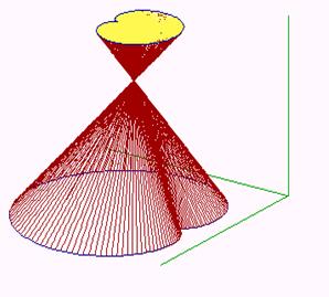
Fig. 11

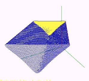
Fig. 12

The first differential form of the homothetical solid is

j₁(u, v, w) = (p_u(u, v) .H(w) du + p_v(u, v) .H(w) dv + p(u, v) .H´(w) dw)²=

= (1-kw)² (x_u² + y_u² + z_u²) du² + (1-kw)²(x_v² + y_v² + z_v²) dv² +

+ k²((x -a)² + (y -b)² + (z -c)²) dw² + 2(1-kw)²(x_u x_v+ y_u y_v + z_u z_v) du dv -

-2k(1-kw)(x_u(x-a) + y_u(y-b) + z_u(z-c)) du dw -

- 2k(1-kw)(x_v(x -a) + y_v(y-b) + z_v(z-c )) dv dw

For the coefficient k=1 of the class of homotheties we speak about a cone with the concerned basic surface patch (resp. about a pyramid in the case of a basic n-gon) with the vertex in the point V. For k>1 the doubled cone (resp. pyramid) can be created, while for k <1 a frustum of the cone (resp. pyramid).

Type 3 . (ordered set of points - curve segments - surface patches - solid cells, interpolation)

Basic figure of this last type of solid creative representations is a discrete ordered set of geometric figures represented analytically by homogeneous coordinates (points and vectors) or point functions of 1 - 3 variables (curve segments, surface patches, solid cells). These form elements of the matrix M(u, v, w) of type nxmxl (map of the basic figure) with respect to the position of the figures in the defined order in three directions in the space.

Generating principle is a set of 1 - 3 approximations (interpolations) represented by interpolation matrices with elements in interpolation polynomials

I(u)=(F₁(u), ..., F_n(u)), I(v)=(F₁(v), ...,F_m(v)), I(w))=(F₁(w), ..., F_l(w))

Created approximation (interpolation) solid cell is analytically represented by the point function

s(u, v, w) = [- I(u). M(u, v, w) . I^T(v)] . I^T(w)

differentiable on the region W = [0,1]³ .

Approximation (interpolation) solid interior can be controlled by the elements of the basic figure, and inhomogeneous solids with respect to all variables u, v, w can be created.